Differences in Terminology and Capability
Building on the terms and concepts introduced in Part I of this white paper, Part II digs deeper into the difference in the meaning of some key terms used in both Property Graphs and Knowledge Graphs, including LABELS, TYPES, and PROPERTIES. Key terms such as these actually mean very different things depending on the graph data model one talks about. This is important to understand in order to avoid confusion.
It is also important to understand in order to appreciate differences in the capabilities that these two graph data models provide. Certain key terms used when describing graphs actually mean very different things depending on the graph data model one talks about. This is important to understand to avoid confusion. It is also important to understand in order to appreciate differences in the capabilities that these two graph data models provide.
We will now describe the differences in the meaning and use of some key concepts—LABELS, TYPES, and PROPERTIES.
What are Labels and Types
In RDF Graphs, a label is a standard predicate defined in the RDFS namespace—rdfs:label. It is used to point to the value of a display name for any resource. For example, the label for resource wikidata:Q6 in the graph shown in Figure 2 is “New York City.” You could also use another predicate for this purpose, but rdfs:label is widely accepted as a unique identifier of a property that connects a resource to its display name. In Property Graphs it is typical to create a property called “name” and use it to hold a display name for a node. You could also use a differently named property.

Click on the image to see a larger version.

Click on the image to see a larger version.
In Property Graphs, the term “label” is used to identify the type of a node. It is called a label rather than a type because it is simply a string—a textual tag. It has no meaning beyond the text. No information about it can be captured in a graph. Edges in a Property Graph also have a tag that identifies the type of an edge. It is called a “type” or, sometimes, “relationship type.” It is used in queries when matching relationships, and it is also used as a display name for edges when graphs are shown visually.
Contrastingly, in RDF Graphs, the type of a node or property’s type is a resource i.e., another node in the graph—typically, with additional information associated with it to define its intended use and semantics. A node is connected to its type using the rdf:type predicate.
Note that some Property Graph databases (e.g., SAP Hana) do not use the term “label” at all and, instead use the term “type” or “node type.” The underlying implementation, however, is the same—type is a tag for a node or a tag for a property. It is not a node itself.
Let’s take a look in Figure 3, at a fragment of the same RDF graph we showed in Figure 2, now expanded with more information about types or classes and other schema elements.

Click on the image to see a larger version.
The green border around nodes or edges indicates graph elements that describe the data model. In RDF, as in Property Graphs, nodes can belong to more than one set (class). We see this with Actor and Director. Tom Hanks is both. However, if one of the classes is a subclass of another, there is no need in RDF to specify a “parent type.” Instead, this information is provided at the class level for all resources that belong to a class—because class information is also a part of the RDF graph.
For example, unlike the Property Graph in Figure 1, we do not say in Figure 2 that Tom Hanks is a person in addition to being an actor and a director or that Sara Paulson is a person in addition to being an actor. We simply say that there is a rdfs:subClassOf relationship between the class of Actors and the class of People. And the same for the class of Directors. The semantics of rdf:type and rdfs:subClassOf are defined in the standard—the graph depicted in Figure 3 says that every resource of type Actor is also of type Person.
We also do not say that the type of New York City or White Plains is a place (location) in addition to a city. We do not need to repeat this fact for each city. We already said it in the model—each city is also a place and what is defined for a place will apply to a city.
In an RDF Graph, we can capture any information about the model of the data that is stored in a graph. This information will be stored, accessed, and processed the same way as any other data. For example, the graph diagram in Figure 3 shows that we can add a label to the predicate ex:actedIn. Similarly, we could also say that when the relationship ex:actedIn is used to navigate in the opposite direction (from a movie to an actor), the display name of the relationship should be shown as ‘actors.’ In an RDF Graph, a resource that is used as a predicate in one statement can be used as a subject or object in another statement. This is an example of the additional flexibility that, among other things, lets us store information about predicates and their usage. The edges in Property Graphs offer nothing comparable.
We can extend the RDF graph further to explicitly define how a predicate should be used. For example, we could say that any resource of type schema:CreativeWork can have a property ex:released and the value of that property must be a date. This would apply to a Movie or a TV Series since they both are subclasses of schema: Creative- Work. The diagram in Figure 4 shows what this looks like in a graph.
In Figure 4, the sh: prefix (e.g. in sh:property) stands for w3.org/ns/shacl#, the standard namespace that is used for SHACL—a language for defining rules and constraints for RDF Graphs, turning them into fully fledged Knowledge Graphs. SHACL offers a very strong approach to ensuring the integrity of RDF data and more.
For instance, we can:
- Consult a graph to find out what properties are appropriate for, let’s say, a movie and what are the valid values for these properties.
- Define constraints also known as rich data quality/validity rules. For example, as shown in Figure 4, we have defined a min range of allowed date values for the ‘re- leased’ property of a creative work (e.g., a movie or a TV Series). Now, if a movie released prior to 1900 is added to a graph, the graph can identify it as a problem. While this example is simple, we can add to the graph much more sophisticated rules. For instance, we could specify copy- right regulations that must be in place for resources released or published after a certain date
- Define rich inference rules. Inference rules generate new facts from the facts in the graph.
These key capabilities turn RDF Graphs into Knowledge Graphs.

about the ex:released property.
Click on the image to see a larger version.
What are Properties
In RDF Graphs, an edge is called a property (predicate) and an object that a property points to may be called a property value. All property values (literals and URIs alike) are stored as nodes. For example, as shown in Figure 2:
- The rdfs:label for the resource ex:125 is “The Post.” In this example, rdfs:label is a property and “The Post” is a value.
- The edge ex:filmedIn is also a property. Its values for ex:125 are wikidata:Q6 and wikidata:Q462177.
- In “data modeling speak,” in an RDF Graph property can be either attributes or relationships.
In Property Graphs, properties can only have literal values. These are stored and treated differently from the nodes in a graph. In data modeling speak, properties in a Property Graph are always attributes. This is why property graphs are formally described as directed, edge labeled, attributed graphs.
A property structure is that of key-value pairs. This means that a property key can only have a single value. If it has more than one value, then the single value is turned into an array of comma separated values. For an
example, see Figure 5.

key-value pairs—multiple values must be turned into an array of comma separated values
Click on the image to see a larger version.
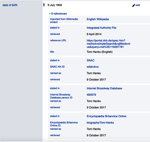
Turning multi-valued properties into arrays makes it harder to efficiently answer queries such as “all cities with population over 58,000.” The first value in the array is the population of White Plains in 2018. The second value is the population of White Plains in 2010. There is no way in a Property Graph to capture what each of these values represents beyond the fact that the key part of the key-value pair is Population. This brings us to the next important difference—how to capture additional information about a property value. In saying this, we mean any property—whether it is an attribute or a relationship. As we see with the population example, it may be important to qualify a measurement by the date it was measured on. There are also other important information qualifiers—including source and confidence. For example, Wikidata captures many details about the source of the information about Tom Hanks’ birth date in order to give users confidence in the reliability of the data. As shown in Figure 6, it got the information from 9 sources which all agree on the date. The sources include the Encyclopedia Britannica, Internet Broadway Database, and others.
Click on the image to see a larger version.
Differences in Attaching Information about an Edge
In RDF Graphs, unlike in Property Graphs, edges are typically re-used:
- In the Property Graph shown in Figure 1, there are two ACTED_IN edges with different IDs: an edge connecting the node representing Tom Hanks to the node representing the movie The Post and an edge connecting Sarah Paulson to this movie. The two edges have the same type, but different identity.
- In RDF, it is the same edge. This means that if you need to say something about a relationship between Tom Hanks and The Post (e.g., the role he played in the movie), you can’t simply add a statement to the ex:actedIn property. If you do this, it will apply everywhere this property is used.
In other words, in the Property Graph data model, edges uniquely identify the sourcenode — edge — target-node combination. In the RDF data model, they tend not to. Of course, one could create a unique edge and simply give it the type ex:actedIn. However, this is normally not done because RDF databases are optimized for working with edges that represent types instead of occurrences of types.
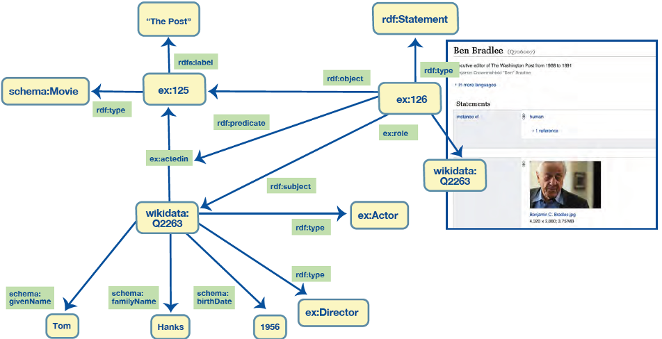
To support the need to attach information on an edge between two specific nodes, RDF provides a way to create a new node that uniquely identifies the source-edge-target triple (or the subject-predicate-object in RDF speak) combination. With that in place, we can make statements about the new node using the regular approach—it can be a subject or an object of any statement. This is shown in Figure 7 where we created a new node ex:126 to represent the statement (triple) of Tom Hanks’ acting in The Post. The new node is connected to the statement about Tom’s acting in The Post using rdf:subject, rdf:predicate, rdf:object and rdf:Statement, built-in elements of the RDF data model that support this use case.
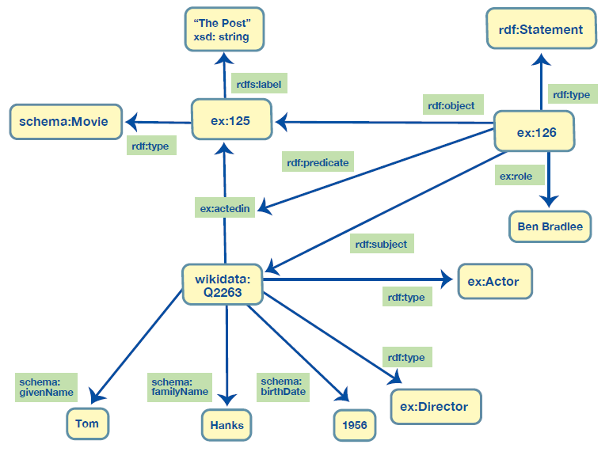
statement—to attach information on an edge between two specific nodes
Click on the image to see a larger version.
Compared to Property Graphs, this approach is more powerful and flexible because it supports:
- Adding other edges (relationships) to edges. For example, instead of having a role as a string, we may want to have a connection to a node representing Ben Bradlee, a person. This is fundamentally not possible with Property Graphs without changing (restructuring) the original graph.
- Adding more information to any property, not just a relationship. For example, we can use it to specify the effective date of each population measurement for White Plains. This is also not possible with Property Graphs.
For Property Graphs, the solution to the need to add edges to other edges is to create intermediate nodes—as shown in Figure 8. This requires restructuring of a graph and changing all queries and logic because the path between actors and movies is now different (compare with the original graph in Figure 1).
With RDF, you do not need to make changes to the graph structure to make a link to the resource representing Ben Bradlee. You simply change the node at the end of the ex:role relationship from a string to a URI. This is demonstrated in Figure 8. The approach is evolutionary and does not require any refactoring other than the change of the value itself.
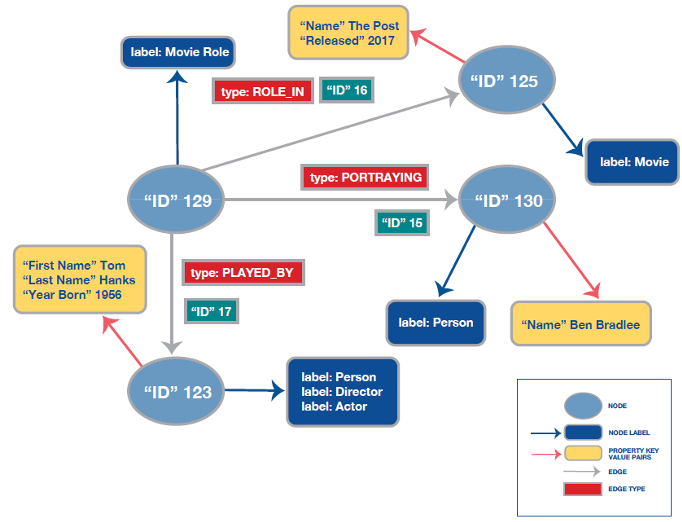
with Ben Bradlee as a Person
Click on the image to see a larger version.
There may, however, be some other situations where you would want to introduce new intermediate nodes. If you do so, SHACL rules can be used to deliver the original relationship path inferring its value from the new, more complex path. In this way, your existing queries and programs can remain the same.
The Property Graph solution to adding more information to a property (e.g., population) is to change the structure of the graph to turn a property into an edge and a value to a node. This requires restructuring of a graph and change to all queries and logic for its processing because the storage and access of properties is fundamentally different and separate from the graph traversal. This makes Property Graphs less evolvable or flexible than RDF Graphs.
Flexibility is acknowledged as the key differentiating advantage of graph databases. For example, the leading vendor of property graph databases says, “With graph databases, IT and data architect teams move at the speed of business because the structure and schema of a graph model flexes as applications and industries change. Rather than exhaustively modeling a domain ahead of time, data teams can add to the existing graph structure without endangering current functionality.” We agree that this would be a very important and desired advantage. However, as we describe in this paper, changes in the model of the Property Graph data will require refactoring and changes to queries. In a Property Graph edges and properties are different data structures and their handling in queries is fundamentally different.
As you can see, compared to an RDF Graph, it is harder to organically grow a Property Graph in response to changes in your information requirements. A current downside of the RDF Statement approach to capturing information about edges is what is sometimes called “graph bloat.” To capture a role that Tom Hanks had in The Post, we need to add at least three extra statements (rdf:subject, rdf:predicate and rdf:object) in addition to the role information—four if you also add a type link to rdf:Statement. Quite a lot of overhead for just one fact. If, however, you need to capture several facts about Tom’s acting in this movie, then this approach has less overhead. A new extension to the RDF data model called RDF* (RDF Star) and its variation called RDF Plus address this issue. It is currently in the process of being added to the standard.
Part II of “Knowledge Graphs vs. Property Graphs” examined in more detail the difference in meaning of some key terms—LABELS, TYPES, and PROPERTIES—used in both Property Graphs and Knowledge Graphs. It also noted significant differences in capabilities resulting from these differences.
Regarding labels and types, we learned that:
- In RDF Graphs, a label is a standard predicate defined in the RDFS namespace—rdfs:label. It is used to point to the value of a display name for any resource.
- In Property Graphs, the term “label” is used to identify the type of a node. It is called a label rather than a type because it is simply a string—a textual tag. It has no meaning beyond the text.
- Contrastingly, in RDF Graphs, the type of a node or property’s type is a resource i.e., another node in the graph—typically, with additional information associated with it to define its intended use and semantics.
Regarding properties, we learned that:
- In Property Graphs, properties can only have literal values. These are stored and treated differently from the nodes in a graph. In data modeling speak, properties in a Property Graph are always attributes.
- In RDF Graphs, an edge is called a property (predicate) and an object that a property points to may be called a property value. All property values (literals and URIs alike) are stored as nodes.
We also learned that Knowledge Graphs:
- Provide a more powerful and flexible way to attached information about an edge in the graph making it easier to organically grow a Knowledge Graph in response to changes in information requirements.
- Can capture any information about the model of the data that is stored in a graph.
- Are easily extended to explicitly define how a predicate should be used, with SHACL — a language for defining rules and constraints for RDF Graphs.
